1 Régression simple

La concentration en ozone

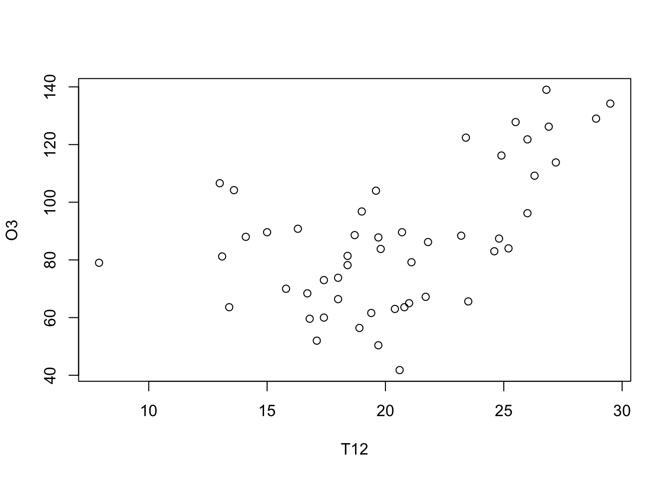
ozone <- read.table("../donnees/ozone_simple.txt",header=TRUE,sep=";")
plot(O3~T12, data=ozone, xlab="T12", ylab="O3")

reg <- lm(O3~T12, data=ozone)
summary(reg)

Call:
lm(formula = O3 ~ T12, data = ozone)

Residuals:
    Min      1Q  Median      3Q     Max 
-45.256 -15.326  -3.461  17.634  40.072 

Coefficients:
            Estimate Std. Error t value Pr(>|t|)    
(Intercept)  31.4150    13.0584   2.406     0.02 *  
T12           2.7010     0.6266   4.311 8.04e-05 ***
---
Signif. codes:  0 '***' 0.001 '**' 0.01 '*' 0.05 '.' 0.1 ' ' 1

Residual standard error: 20.5 on 48 degrees of freedom
Multiple R-squared:  0.2791,    Adjusted R-squared:  0.2641 
F-statistic: 18.58 on 1 and 48 DF,  p-value: 8.041e-05

plot(O3~T12, data=ozone)
T12 <- seq(min(ozone[,"T12"]), max(ozone[,"T12"]), length = 100)
grille <- data.frame(T12)
ICdte <- predict(reg, new=grille, interval="conf", level=0.95)
matlines(grille$T12, cbind(ICdte), lty = c(1,2,2), col = 1)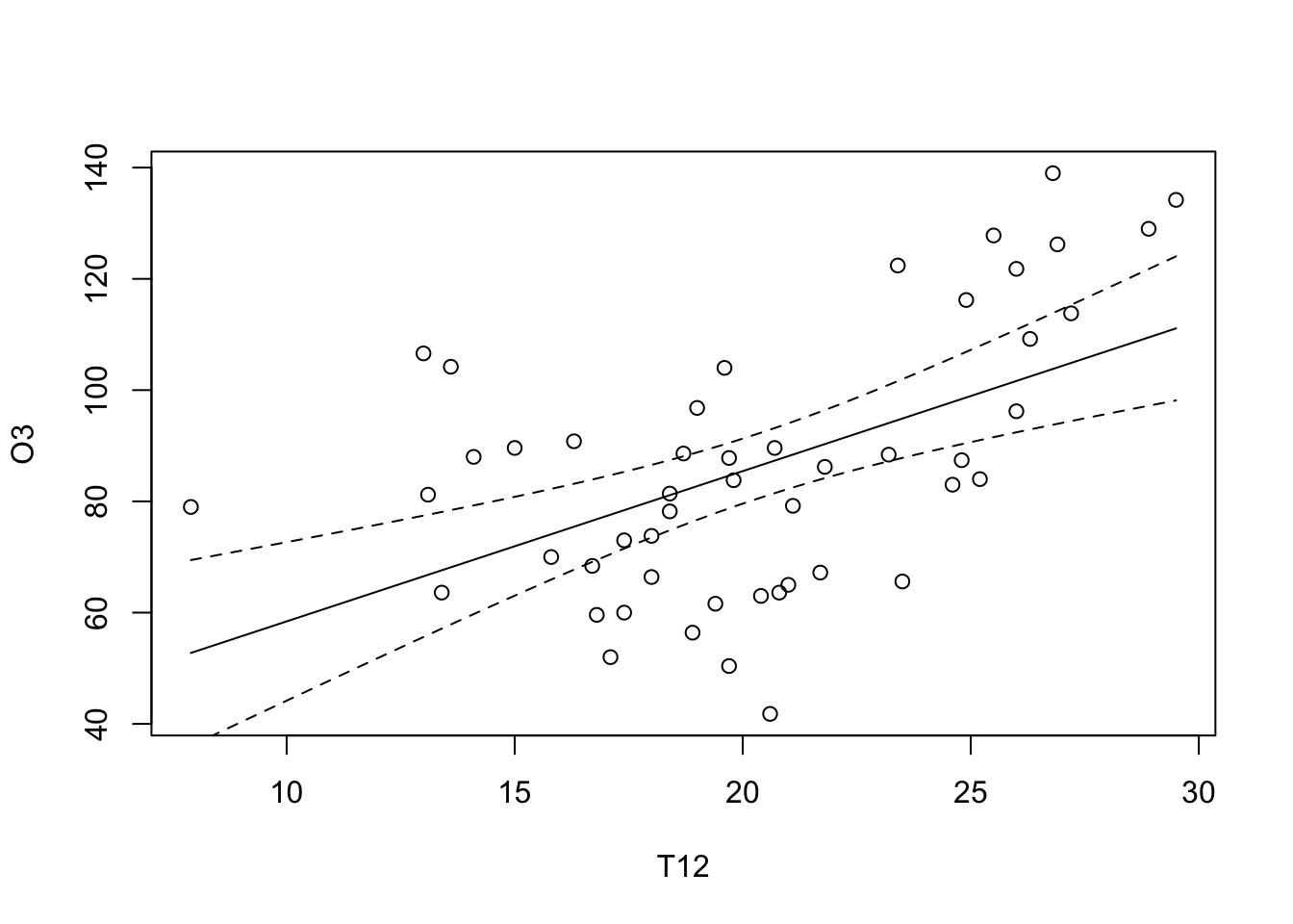

plot(O3~T12, data = ozone, ylim = c(0,150))
T12 <- seq(min(ozone[,"T12"]), max(ozone[,"T12"]), length = 100)
grille <- data.frame(T12)
ICdte <- predict(reg, new=grille, interval="conf", level=0.95)
ICprev <- predict(reg, new=grille, interval="pred", level=0.95)
matlines(T12, cbind(ICdte,ICprev[,-1]), lty=c(1,2,2,3,3), col=1)
legend("topleft", lty=2:3, c("Y","E(Y)"))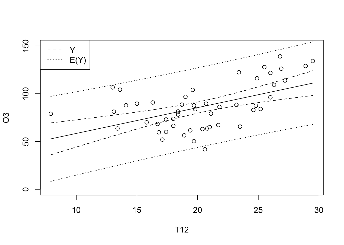

IC <- confint(reg, level = 0.95)
IC

               2.5 %   97.5 %
(Intercept) 5.159232 57.67071
T12         1.441180  3.96089

library(ellipse)
plot(ellipse(reg, level=0.95), type = "l", xlab = "", ylab = "")
points(coef(reg)[1], coef(reg)[2], pch = 3)
lines(IC[1,c(1,1,2,2,1)], IC[2,c(1,2,2,1,1)], lty = 2)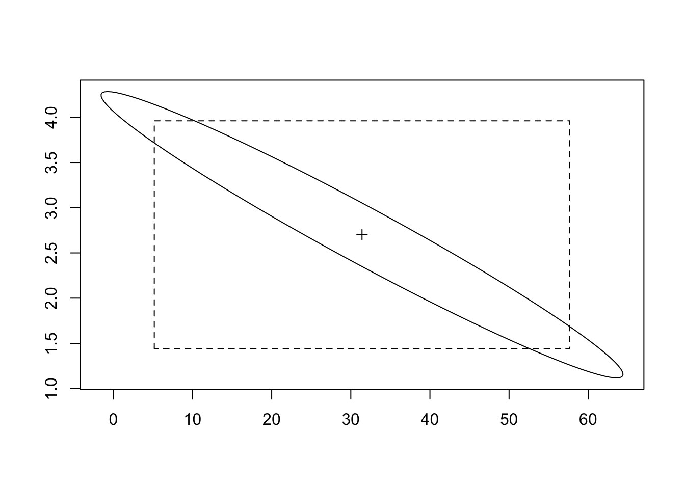

La hauteur des eucalyptus

eucalypt <- read.table("../donnees/eucalyptus.txt", header = T, sep = ";")
plot(ht~circ, data = eucalypt, xlab = "circ", ylab = "ht")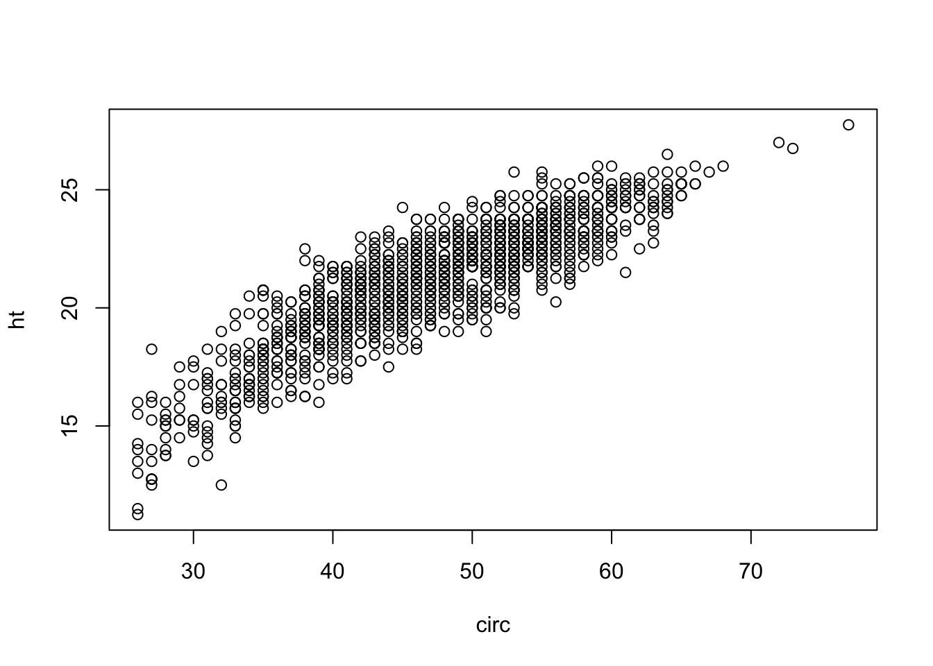

reg <- lm(ht~circ, data = eucalypt)
summary(reg)

Call:
lm(formula = ht ~ circ, data = eucalypt)

Residuals:
    Min      1Q  Median      3Q     Max 
-4.7659 -0.7802  0.0557  0.8271  3.6913 

Coefficients:
            Estimate Std. Error t value Pr(>|t|)    
(Intercept) 9.037476   0.179802   50.26   <2e-16 ***
circ        0.257138   0.003738   68.79   <2e-16 ***
---
Signif. codes:  0 '***' 0.001 '**' 0.01 '*' 0.05 '.' 0.1 ' ' 1

Residual standard error: 1.199 on 1427 degrees of freedom
Multiple R-squared:  0.7683,    Adjusted R-squared:  0.7682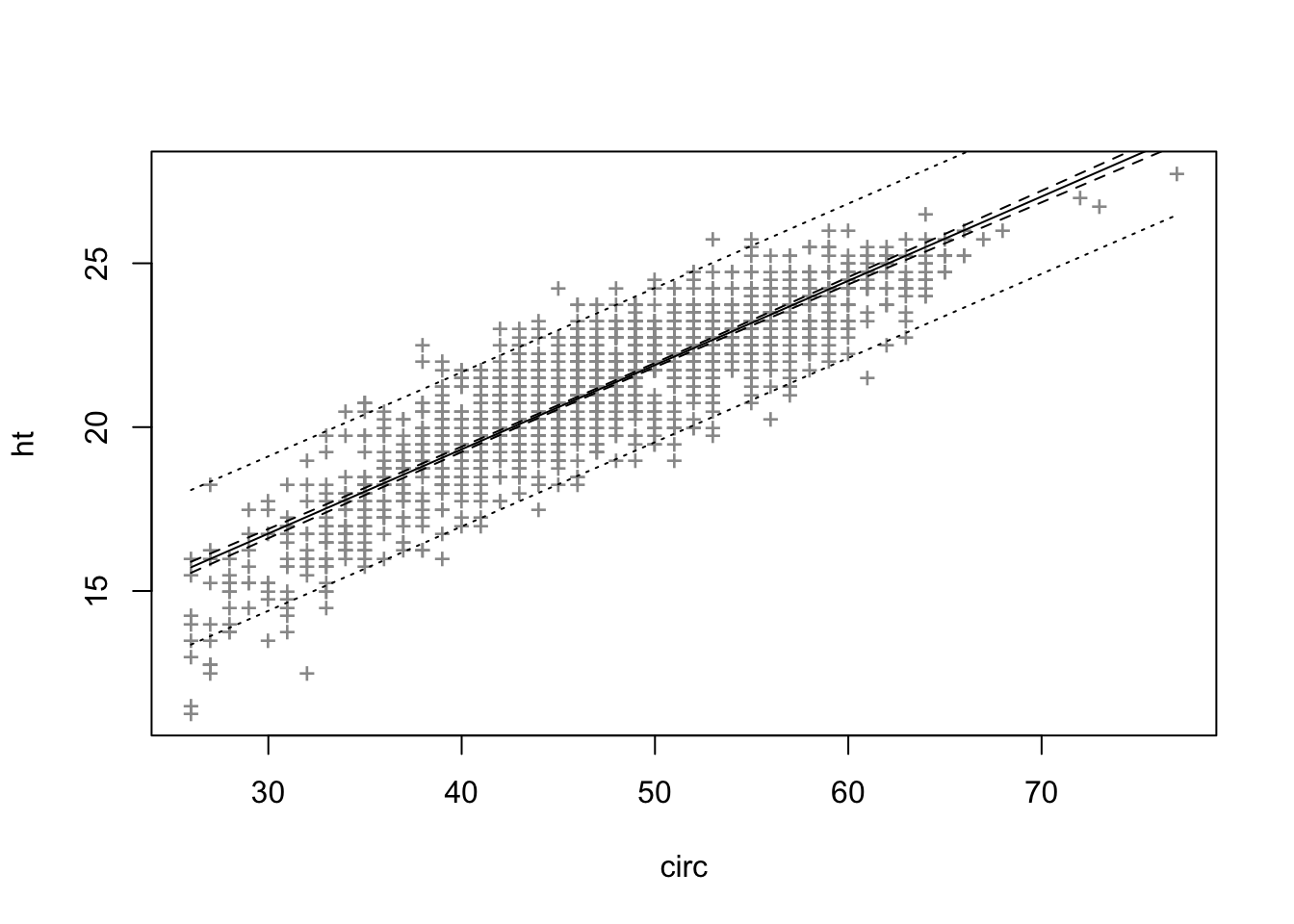 
F-statistic:  4732 on 1 and 1427 DF,  p-value: < 2.2e-16

plot(ht~circ, data = eucalypt, pch = "+", col = "grey60")
grille <- data.frame(circ = seq(min(eucalypt[,"circ"]),
                                max(eucalypt[,"circ"]), length = 100))
ICdte <- predict(reg, new=grille, interval="confi", level=0.95)
matlines(grille$circ, ICdte, lty = c(1,2,2), col = 1)

plot(ht~circ, data = eucalypt, pch = "+", col = "grey60")
circ <- seq(min(eucalypt[,"circ"]),max(eucalypt[,"circ"]), len = 100)
grille <- data.frame(circ)
Cdte <- predict(reg, new=grille, interval="conf", level=0.95)
ICprev <- predict(reg, new=grille, interval="pred", level=0.95)
matlines(circ, cbind(ICdte,ICprev[,-1]),lty=c(1,2,2,3,3), col=1)