14 Comparaison en classification supervisée

Exercice 1 (Questions de cours) C, D, A, B.

Exercice 2 (Règle de Bayes)

1. La règle de Bayes est définie par \[% g^\star(x)=\left\{ \begin{array}{ll} 1& \text{si }\mathbf P(Y=1|X=x)\geq 0.5 \\ 0& \text{sinon.} \end{array}\right. \] L’erreur de Bayes est définie par $L^\star=\mathbf P(g^\star(X)\neq Y)$.
2. On a \[% \begin{aligned} \mathbf P(g(X)\neq Y|X=x) & = 1-\Big(\mathbf P(g(X)=Y,g(X)=1|X=x) \\ & \hspace{2cm}+\mathbf P(g(X)=Y,g(X)=0|X=x)\Big) \\ & = 1-\Big(\mathbf 1_{g(x)=1}\mathbf P(Y=1|X=x) \\ & \hspace{2cm}+\mathbf 1_{g(x)=0}\mathbf P(Y=0|X=x)\Big) \\ & = 1-(\mathbf 1_{g(x)=1}\eta(x)+\mathbf 1_{g(x)=0}(1-\eta(x))). \end{aligned} \]
3. On déduit \[% \begin{aligned} \mathbf P( g(X)\neq Y|X=x)-\mathbf P(g^\star(X)\neq Y|X=x) & = \eta(x)\left(\mathbf 1_{g^\star(x)=1}-\mathbf 1_{g(x)=1}\right)+(1-\eta(x))\left(\mathbf 1_{g^\star(x)=0}-\mathbf 1_{g(x)=0}\right) \\ & = \eta(x)\left(\mathbf 1_{g^\star(x)=1}-\mathbf 1_{g(x)=1}\right)+(1-\eta(x))\left(1-\mathbf 1_{g^\star(x)=1}-(1-\mathbf 1_{g(x)=1})\right) \\ & = (2\eta(x)-1) \left(\mathbf 1_{g^\star(x)=1}-\mathbf 1_{g(x)=1}\right) \\ \end{aligned} \]
- Quand le premier terme $(2\eta(x)-1)$ est positif cela signifie que $\eta(x)=\mathbf P(Y|=1X=x)\geq 0.5$. Par définition de $g^\star$ nous en déduisons donc que $g^\star(x)=1$ et donc que le second terme est aussi positif ou nul.
- Quand le premier terme $(2\eta(x)-1)$ est négatif cela signifie que $\eta(x)=\mathbf P(Y|=1X=x)< 0.5$. Par définition de $g^\star$ nous en déduisons donc que $g^\star(x)=0$ et donc que le second terme est aussi négatif ou nul.
  En conclusion nous avons bien que \[% \mathbf P(g(X)\neq Y|X=x)-\mathbf P(g^\star(X)\neq Y|X=x) = (2\eta(x)-1) \left(\mathbf 1_{g^\star(x)=1}-\mathbf 1_{g(x)=1}\right) \geq 0 \]
1. On conclut en intégrant par la loi de $X$ que \[% \mathbf P(g(X)\neq Y)\geq \mathbf P(g^\star(X)\neq Y). \]
Pour la règle de Bayes, on a
- si $x\leq 0$, on a $\mathbf P(Y=1|X=x)=\mathbf P(U\leq 2)=\frac{1}{5}$ $\Longrightarrow$ $g^\star(x)=0$.
- si $x> 0$, on a $\mathbf P(Y=1|X=x)=\mathbf P(U> 2)=\frac{9}{10}$ $\Longrightarrow$ $g^\star(x)=1$.
L’erreur de Bayes vaut \[% \begin{aligned} L^\star=\mathbf P(g^\star(X)\neq Y& |X\leq 0)\mathbf P(X\leq 0) \\ & +\mathbf P(g^\star(X)\neq Y|X> 0)\mathbf P(X>0). \end{aligned} \] Or \[% \mathbf P(g^\star(X)\neq Y|X\leq 0)=\mathbf P(Y\neq 0|X\leq 0)=\frac{1}{5} \] et \[% \mathbf P(g^\star(X)\neq Y|X> 0)=\mathbf P(Y\neq 1|X> 0)=\frac{1}{10}. \] On obtient \[%L^\star=\frac{1}{5}\,\frac{1}{2}+\frac{1}{10}\,\frac{1}{2}=\frac{3}{20}.\]

Exercice 3 (Fonctions R)

Exercice 4 (Score aléatoire) Il suffit d’utiliser l’indépendance entre $S(X)$ et $Y$ : \[ \begin{aligned} x(s)= & \mathbf P(S(X)> s|Y=0)=\mathbf P(S(X)> s)=\mathbf P(S(X)\geq s) \\ =& \mathbf P(S(X)\geq s|Y=1)=y(s), \end{aligned} \]

Exercice 5 (Score parfait et courbe ROC) Nous prendrons un score variant entre $-\infty$ et $+\infty$. Si le score est issu d’une probabilité il variera entre $0$ et $1$ et il suffira de remplacer $-\infty$ par 0 et $+\infty$ par 1 dans le calculs qui suivent. Le score est parfait et nous avons donc un seuil $s^\star$ tel que - si $S(x)\leq s^\star$ nous avons forcément $Y=0$ et réciproquement. Autrement dit $\mathbf P(Y=0|S(x)\leq s^\star)=1$ et $\mathbf P(S(X)\leq s^\star|Y=0)=1$ - et aussi dans l’autre sens si $S(x)> s^\star$ nous avons forcément $Y=1$ et réciproquement. Autrement dit $\mathbf P(Y=1|S(x)> s^\star)=1$ et $\mathbf P(S(X)> s^\star|Y=1)=1$.

Analysons la courbe paramétrée en ce point: $s^\star$. On a ici pour l’abscisse \[% \begin{align*} x(s^\star)= & \mathbf P(S(X)> s^\star|Y=0) \\ =&1 - \mathbf P(S(X)\geq s^\star | Y=0)\\ =& 1-1 =0. \end{align*} \]

Calculons l’ordonnée: \[% \begin{aligned} y(s^\star)=&\mathbf P(S(X)\geq s^\star|Y=1)= 1-\mathbf P(S(X)\leq s^\star|Y=1) \\ =&1- \frac{\mathbf P(S(X)\leq s^\star\cap Y=1)}{\mathbf P(Y=1)}\\ =&1- \frac{\mathbf P(Y=1| S(X)\leq s^\star)\mathbf P(S(X)\leq s^\star) }{\mathbf P(Y=1)} \\ =&1- \frac{(1-\mathbf P(Y=0| S(X)\leq s^\star))\mathbf P(S(X)\leq s^\star) }{\mathbf P(Y=1)} \\ =&1 -0=1 \end{aligned} \] puisque $\mathbf P(Y=0| S(X)\leq s^\star)=1.$

Conlusion: en $s^\star$ la courbe est au point $M=(1,0)$.
Plaçons nous en une valeur $s>s^\star.$ Puisque $s>s^\star$ nous avons forcément que que quand $S(X)>s$ on a $Y=1$ et donc $\mathbf P(Y=1| S(X)> s)=0.$ \[% \begin{aligned} x(s)= & \mathbf P(S(X)> s|Y=0) \\ =&\frac{\mathbf P(S(X)> s\cap Y=0)}{\mathbf P(Y=0)}\\ =& \frac{\mathbf P(Y=0| S(X)> s)\mathbf P(S(X)> s) }{\mathbf P(Y=0)} \\ =& \frac{(1-\mathbf P(Y=1| S(X)> s))\mathbf P(S(X)> s) }{\mathbf P(Y=0)}=0 \end{aligned} \] Pour l’ordonnée nous avons que \[% \begin{aligned} y(s)=&\mathbf P(S(X)\geq s|Y=1)= 1-\mathbf P(S(X)\leq s|Y=1) \end{aligned} \] Comme $prob(S(X)\leq s|Y=1)$ est une fonction de répartition nous avens donc que $\lim_{s\rightarrow+\infty}prob(S(X)\leq s|Y=1)=1$ et donc que \[% \begin{aligned} \lim_{s\rightarrow+\infty}y(s)=&0 \end{aligned} \] Conclusion: pour $s\geq s^\star$ l’abscisse vaut toujours 0 et l’ordonnée tend vers 0. Donc quand $s\in[s^\star, +\infty[$ le point $(x(s),y(s))$ parcourt le segment $[O,M]$.
Plaçons nous dans le cas où $s<s^\star$. Dans ce cas nous avons que l’évènement $\{S(X)\geq s^\star|Y=1\} \subset\{S(X)\geq s|Y=1\}$ et donc \[% \begin{aligned} y(s)=&\mathbf P(S(X)\geq s|Y=1)\geq \mathbf P(S(X)\geq s^\star|Y=1)=1 \end{aligned} \] De plus nous avons que \[% \begin{aligned} x(s)=&\mathbf P(S(X)> s|Y=0)= 1-\mathbf P(S(X)\leq s|Y=0) \end{aligned} \]

Comme $prob(S(X)\leq s|Y=0)$ est une fonction de répartition nous avens donc que $\lim_{s\rightarrow-\infty}prob(S(X)\leq s|Y=0)=0$ et donc que \[% \begin{aligned} \lim_{s\rightarrow-\infty}x(s)=&1 \end{aligned} \] Conclusion: pour $s\leq s^\star$ l’ordonnée vaut toujours 1 et l’absicsse tend vers 0. Donc quand $s\in]- \infty , s^\star]$ le point $(x(s),y(s))$ parcourt le segment $[M, (1,1)]$.

Exercice 6 (Score parfait et courbe lift) Nous prendrons un score variant entre $-\infty$ et $+\infty$. Si le score est issu d’une probabilité il variera entre $0$ et $1$ et il suffira de remplacer $-\infty$ par 0 et $+\infty$ par 1 dans le calculs qui suivent. Le score est parfait et nous avons donc un seuil $s^\star$ tel que - si $S(x)\leq s^\star$ nous avons forcément $Y=0$ ou autrement dit $\mathbf P(Y=0|S(x)\leq s^\star)=1$; - et aussi dans l’autre sens si $S(x)> s^\star$ nous avons forcément $Y=1$ ou autrement dit $\mathbf P(Y=1|S(x)> s^\star)=1$.

Analysons la courbe paramétrée en ce point: $s^\star$. On a ici pour l’abscisse \[% \begin{align*} x(s^\star)= & \mathbf P(S(X)> s^\star) = \mathbf P(S(X)> s^\star \cap Y=0) + \mathbf P(S(X)> s^\star \cap Y=1)\\ = & \mathbf P(S(X)> s^\star | Y=0)\mathbf P(Y=0) + \mathbf P(S(X)> s^\star | Y=1)\mathbf P(Y=1) \end{align*} \] Comme le score est parfait nous avons que $\mathbf P(S(X)> s^\star | Y=0)=0$ et $\mathbf P(S(X)> s^\star | Y=1)=1$ d’où la conclusion \[% \begin{aligned} x(s^\star)= \mathbf P(Y=1) \end{aligned} \]

Calculons maintenant l’ordonnée: \[% \begin{aligned} y(s^\star)=&\mathbf P(S(X)\geq s^\star |Y=1)=1 \end{aligned} \] puisque le score est parfait.$

Conlusion: en $s^\star$ la courbe est au point $M=(\mathbf P(Y=1),1)$.
Plaçons nous en un point $s\geq s^\star$. L’abscisse vaut \[% \begin{aligned} x(s)= & \mathbf P(S(X)> s) \end{aligned} \] et l’ordonnée \[% \begin{aligned} y(s)=&\mathbf P(S(X)\geq s |Y=1) = \frac{\mathbf P(S(X)\geq s \cap Y=1)}{\mathbf P(Y=1)} \end{aligned} \] Comme le score est parfait nous avons en $s\geq s^\star$ \[% \begin{aligned} \mathbf P( Y=1|S(X)\geq s) &= 1\\ \mathbf P( Y=0|S(X)\geq s) &= 0\\ \frac{\mathbf P(S(X)\geq s \cap Y=0)}{\mathbf P(S(X)\geq s )}&=0\\ \mathbf P(S(X)\geq s \cap Y=0)&=0 \end{aligned} \] nous pouvons donc ajouter $\mathbf P(S(X)\geq s \cap Y=0)$ et obtenir \[% \begin{aligned} y(s)=& \frac{\mathbf P(S(X)\geq s \cap Y=1) + \mathbf P(S(X)\geq s \cap Y=0)}{\mathbf P(Y=1)}= \frac{\mathbf P(S(X)\geq s)}{\mathbf P(Y=1)}\\ &=\frac{x(s)}{\mathbf P(Y=1)} \end{aligned} \] On en déduit donc que le coefficient directeur de la droite est $1/\mathbf P(Y=1)$ et qu’elle passe par le point $(x(s^\star), y(s^\star))$. Trouvons maintenant le point quand $s\rightarrow+\infty$. Nous savons que $x(s)=\mathbf P(S(X)> s)=1-\mathbf P(S(X)\geq s)$ et que $prob(S(X)\geq s)$ est une fonction de répartition, nous avons donc que $\mathbf P(S(X)\geq s)\rightarrow+1$ et donc que $x(s)\rightarrow 0$. Comme $y(s)=x(s)/\mathbf P(Y=1)$ on en déduit que $y(s)\rightarrow 0$. Conlusion: entre $s^\star$ et $+\infty$ le point $(x(s), y(s))$ parcours le segment $(x(s^\star), y(s^\star))$ $(0,0)$.
1. Quand $s= s^\star$ le score parfait on a \[% \begin{aligned} y(s^\star)=&\mathbf P(S(X)\geq s^\star |Y=1)=1 \end{aligned} \] Si nous avons $s\leq s^\star$ l’évènement le score est plus grand que $s$ contient forcément l’évènement le score est plus grand que $s^\star$ et donc en en déduit que \[% \begin{aligned} y(s)=&\mathbf P(S(X)\geq s|Y=1)\geq \mathbf P(S(X)\geq s^\star|Y=1)=1 \end{aligned} \] Donc puisqu’il s’agit d’une probabilité nous avons $y(s)=1 \ \forall s\leq s^\star$. Par ailleurs l’abscisse est par définition \[% \begin{aligned} x(s)= & \mathbf P(S(X)> s) = 1 - \mathbf P(S(X)\leq s) \end{aligned} \] et quand $s\rightarrow-\infty$ la fonction de répartition tend vers 0 et donc $x(s)\rightarrow 1$

Exercice 7 (Calculs de scores avec R)

On propose d’utiliser la version empirique de \[ AUC(S)=\mathbf P(S(X_1)\geq S(X_2)|(Y_1,Y_2)=(1,-1)), \] c’est-à-dire d’estimer l’AUC en calculant, parmi les paires qui vérifient $(Y_1,Y_2)=(1,-1)$, la proportion de paires qui vérifient $S(X_1)\lt S(X_2)$. Si on note \[ \mathcal I=\{(i,j),y_i=1,y_j=0\}, \] alors l’estimateur s’écrit \[ \widehat{AUC}(S)=\frac{1}{|\mathcal I|}\sum_{(i,j)\in\mathcal I}\mathbf 1_{S(X_i)>S(S_j)}. \]

On importe les données

df <- read.csv("../donnees/logit_ex6.csv")

set.seed(1234)
ind_app <- sample(nrow(df),300)
dapp <- df[ind_app,]
dtest <- df[-ind_app,]

logit <- glm(Y~.,data=dapp,family="binomial")

score <- predict(logit,newdata=dtest,type="response")

D0 <- which(dtest$Y==0)
D1 <- which(dtest$Y==1)
score0 <- score[D0]
score1 <- score[D1]
score.01 <- expand.grid(S0=score0,S1=score1)
mean(score.01$S1>score.01$S0)

[1] 0.7385817

pROC::roc(dtest$Y,score)


Call:
roc.default(response = dtest$Y, predictor = score)

Data: score in 104 controls (dtest$Y 0) < 96 cases (dtest$Y 1).
Area under the curve: 0.7386

Exercice 8 (Validation croisée)

Importons les données de détection d’images publicitaires sur internet
```
pub <- read.table("../donnees/ad_data.txt", header = FALSE, sep = ",",
dec = ".", na.strings = "?", strip.white = TRUE)
names(pub)[ncol(pub)] <- "Y"
table(pub$Y)
```
```
   ad. nonad. 
   459   2820 
```
Créons un facteur pour la variable à expliquer en gérant l’ordre des facteurs.
```
pub$Y <- factor(pub$Y, labels=c("1","0"))
pub$Y <- relevel(pub$Y, "0")
pub <- pub[,-(1:4)]
table(pub$Y)
```
```
   0    1 
2820  459 
```
Construisons nos blocs.
- On crée une variable discrète bloc qui donnera les appartenances au bloc (donc des valeurs entre 1 et 10)
- Pour chaque niveau de $Y$, on crée une variable d’appartenance au bloc valant 1, 2, …, 10, 1, 2, …, 10, 1…. Il y a donc par construction autant (ou un de moins) de 1 que de 2, …, que de 10 pour chaque niveau de $Y$. L’appartenance au bloc étant séquentielle ce n’est pas trop souhaitable
- On permute aléatoirement cette variable pour chaque niveau et on affecte ces valeurs aux coordonnées de chaque niveau de $Y$
```
ind0 <- which(pub$Y==0)
ind1 <- which(pub$Y==1)
set.seed(1234)
nbbloc <- 10
bloc <- 1:nrow(pub)
bloc[ind0] <- sample(rep(1:nbbloc, length = length(ind0)))
bloc[ind1] <- sample(rep(1:nbbloc, length = length(ind1)))
```

Probabilité estimée d’une publicité Nous ajustons/estimons chaque modèle sur tous les blocs sauf le $i^e$ et nous calculons les probabilités estimées du label 1 sur le bloc $i$. Ceci est fait pour tous les blocs. Nous rangeons les probabilités estimées dans l’objet SCORE:

library(glmnet)
nomsmodeles <- c("glm", "glmchoix", paste0(rep(c("ridge", "lasso", "elast"), 3), rep(c("", "C", "A"), each=3)))
## resultats des modeles + Y a prevoir
SCORE <- data.frame(matrix(0, length(bloc), length(nomsmodeles)+1))
names(SCORE) <- c("Y",  nomsmodeles)
## premiere colonne la var Y a prevoir
SCORE$Y <- pub$Y
models <- list() # si on veut voir les variables choisies
## VC 10 fold
for(i in 1:nbbloc){
  print(i)
  pubA <- pub[bloc!=i,]
  pubT <- pub[bloc==i,]
  ##Logistique global
  reglog <- glm(Y~.,data=pubA,family="binomial")
  SCORE[bloc==i,"glm"] <- predict(reglog,pubT,type="response")
  ##Logistique choix 
  reg1 <- glm(Y~1,data=pubA,family="binomial")
  choix <- step(reg1,scope=list(lower=formula(reg1),upper=formula(reglog)),trace=0)
  models[[i]] <- formula(choix)
  SCORE[bloc==i,"glmchoix"] <- predict(choix,pubT,type="response")
  ##
  XA <- pub.X[bloc!=i,]
  YA <- pub.Y[bloc!=i]
  XT <- pub.X[bloc==i,]
  ## ridge
  mod <- cv.glmnet(XA,YA,alpha=0,family="binomial")
  SCORE[bloc==i,"ridge"] <- as.vector(predict(mod, XT, "lambda.1se", type="response"))
  ##  lasso
  mod <- cv.glmnet(XA,YA,alpha=1,family="binomial")
  SCORE[bloc==i,"lasso"] <-  as.vector(predict(mod,XT, "lambda.1se", type="response"))
  ##  elast
  mod <- cv.glmnet(XA,YA,alpha=.5,family="binomial")
  SCORE[bloc==i,"elast"] <-  as.vector(predict(mod,XT, "lambda.1se", type="response"))  
  ## ridge  CV class
  mod <- cv.glmnet(XA,YA,alpha=0,family="binomial",type.measure="class")
  SCORE[bloc==i,"ridgeC"] <- as.vector(predict(mod, XT, "lambda.1se", type="response"))
  ## lasso CV class
  mod <- cv.glmnet(XA,YA,alpha=1,family="binomial",type.measure="class")
  SCORE[bloc==i,"lassoC"] <-  as.vector(predict(mod,XT, "lambda.1se", type="response"))  
  ## elast CV class
  mod <- cv.glmnet(XA,YA,alpha=.5,family="binomial",type.measure="class")
  SCORE[bloc==i,"elastC"] <-  as.vector(predict(mod,XT, "lambda.1se", type="response"))
  ## ridge  CV AUC
  mod <- cv.glmnet(XA,YA,alpha=0,family="binomial",type.measure="auc")
  SCORE[bloc==i,"ridgeA"] <- as.vector(predict(mod, XT, "lambda.1se", type="response"))
  ## lasso CV AUC
  mod <- cv.glmnet(XA,YA,alpha=1,family="binomial",type.measure="auc")
  SCORE[bloc==i,"lassoA"] <-  as.vector(predict(mod, XT, "lambda.1se", type="response"))
  ## elast CV AUC
  mod <- cv.glmnet(XA,YA,alpha=.5,family="binomial",type.measure="auc")
  SCORE[bloc==i,"elastA"] <-  as.vector(predict(mod, XT, "lambda.1se", type="response"))
}
saveRDS(SCORE,"../data_aux/scorepubm4_1VC.RDS")

On calcule la courbe ROC On peut utiliser pROC et créer l’objet de classe roc puis sur cet objet calculer l’AUC pour chaque modèle:

library(pROC)
SCORE <- readRDS("../data_aux/scorepubm4_1VC.RDS")
rocCV <- roc(Y~.,data=SCORE)
sort(round(unlist(lapply(rocCV, auc)), 3), decreasing=TRUE)[1:6]

 ridge ridgeC ridgeA elastA lassoA elastC 
 0.982  0.982  0.963  0.963  0.961  0.959

Pour aller plus loin on peut répéter la même procédure 20 fois (en parallèle)

données et cluster

 library(glmnet)
 library(doParallel)
 pub <- read.table("ad_data.txt",header=FALSE,sep=",",dec=".",na.strings = "?",strip.white = TRUE)
 names(pub)[ncol(pub)] <- "Y"
 pub$Y <- factor(pub$Y,labels=c("1","0"))
 pub$Y <- relevel(pub$Y,"0")
 pub <- pub[,-(1:4)]
 ind0 <- which(pub$Y==0)
 ind1 <- which(pub$Y==1)
 ##les 0 sont au début les 1 à la fin
 ##
 bloc <- rep(0,nrow(pub))
 pub.X <- model.matrix(Y~.,data=pub)[,-1]
 pub.Y <- pub[,"Y"]
 niter <- 20
 coredispo <- max(detectCores()-1,1)
 cl <- makeCluster(min(coredispo,niter))
 clusterSetRNGStream(cl,iseed=78)
 registerDoParallel(cl)

boucle Attention, c’est «un peu» long (sur une machine avec plus de 20 coeurs, il faut 1-2 jours)

res <- foreach(j=1:niter) %dopar% {
library(glmnet)
nomsmodeles <- c("glm", "glmchoix", paste0(rep(c("ridge", "lasso", "elast"), 3), rep(c("", "C", "A"), each=3)))
## resultats des modeles + Y a prevoir
SCORE <- data.frame(matrix(0, length(bloc), length(nomsmodeles)+1))
names(SCORE) <- c("Y",  nomsmodeles)
## premiere colonne la var Y a prevoir
SCORE <- data.frame(Y=pub$Y)
nbbloc <- 10
set.seed(1234+j)
bloc[ind0] <- sample(rep(1:nbbloc, length = length(ind0)))
bloc[ind1] <- sample(rep(1:nbbloc, length = length(ind1)))
for(i in 1:nbbloc){
  pubA <- pub[bloc!=i,]
  pubT <- pub[bloc==i,]
  ##Logistique global
  reglog <- glm(Y~.,data=pubA,family="binomial")
  SCORE[bloc==i,"glm"] <- predict(reglog,pubT,type="response")
  ##Logistique choix 
  reg1 <- glm(Y~1,data=pubA,family="binomial")
  choix <- step(reg1,scope=list(lower=formula(reg1),upper=formula(reglog)),trace=0)
  SCORE[bloc==i,"glmchoix"] <- predict(choix,pubT,type="response")
  ##
  XA <- pub.X[bloc!=i,]
  YA <- pub.Y[bloc!=i]
  XT <- pub.X[bloc==i,]
  ## ridge
  mod <- cv.glmnet(XA,YA,alpha=0,family="binomial")
  SCORE[bloc==i,"ridge"] <- as.vector(predict(mod, XT, "lambda.1se", type="response"))
  ##  lasso
  mod <- cv.glmnet(XA,YA,alpha=1,family="binomial")
  SCORE[bloc==i,"lasso"] <-  as.vector(predict(mod,XT, "lambda.1se", type="response"))
  ##  elast
  mod <- cv.glmnet(XA,YA,alpha=.5,family="binomial")
  SCORE[bloc==i,"elast"] <-  as.vector(predict(mod,XT, "lambda.1se", type="response"))  
  ## ridge  CV class
  mod <- cv.glmnet(XA,YA,alpha=0,family="binomial",type.measure="class")
  SCORE[bloc==i,"ridgeC"] <- as.vector(predict(mod, XT, "lambda.1se", type="response"))
  ## lasso CV class
  mod <- cv.glmnet(XA,YA,alpha=1,family="binomial",type.measure="class")
  SCORE[bloc==i,"lassoC"] <-  as.vector(predict(mod,XT, "lambda.1se", type="response"))  
  ## elast CV class
  mod <- cv.glmnet(XA,YA,alpha=.5,family="binomial",type.measure="class")
  SCORE[bloc==i,"elastC"] <-  as.vector(predict(mod,XT, "lambda.1se", type="response"))
  ## ridge  CV AUC
  mod <- cv.glmnet(XA,YA,alpha=0,family="binomial",type.measure="auc")
  SCORE[bloc==i,"ridgeA"] <- as.vector(predict(mod, XT, "lambda.1se", type="response"))
  ## lasso CV AUC
  mod <- cv.glmnet(XA,YA,alpha=1,family="binomial",type.measure="auc")
  SCORE[bloc==i,"lassoA"] <-  as.vector(predict(mod, XT, "lambda.1se", type="response"))
  ## elast CV AUC
  mod <- cv.glmnet(XA,YA,alpha=.5,family="binomial",type.measure="auc")
  SCORE[bloc==i,"elastA"] <-  as.vector(predict(mod, XT, "lambda.1se", type="response"))
  write(paste("rep.",j,"bloc",j),file="progress.txt",append=TRUE)
}
SCORE
}
saveRDS(res,"../data_aux/scorepubm4_20VC.RDS")
stopCluster(cl)

analyse résultats

ffroc  <- function(x) roc(Y~., data=x)
ttm4_20 <- lapply(scorepubm4_20VC, ffroc)

ffauc  <- function(x) unlist(lapply(x, auc))
aucm4_20 <- do.call(rbind, lapply(ttm4_20, ffauc))

print(sort(apply(aucm4_20,2,mean), decreasing=TRUE)[1:6])

    ridge    ridgeC    elastA    ridgeA    lassoA     elast 
0.9800319 0.9792532 0.9631016 0.9626010 0.9590724 0.9537869

nom <- names(sort(apply(aucm4_20,2,mean), decreasing=TRUE)[1:6])
## boxplot
boxplot(aucm4_20[,-1][,c(1,2,5,8,3,6,9,4,7,10)])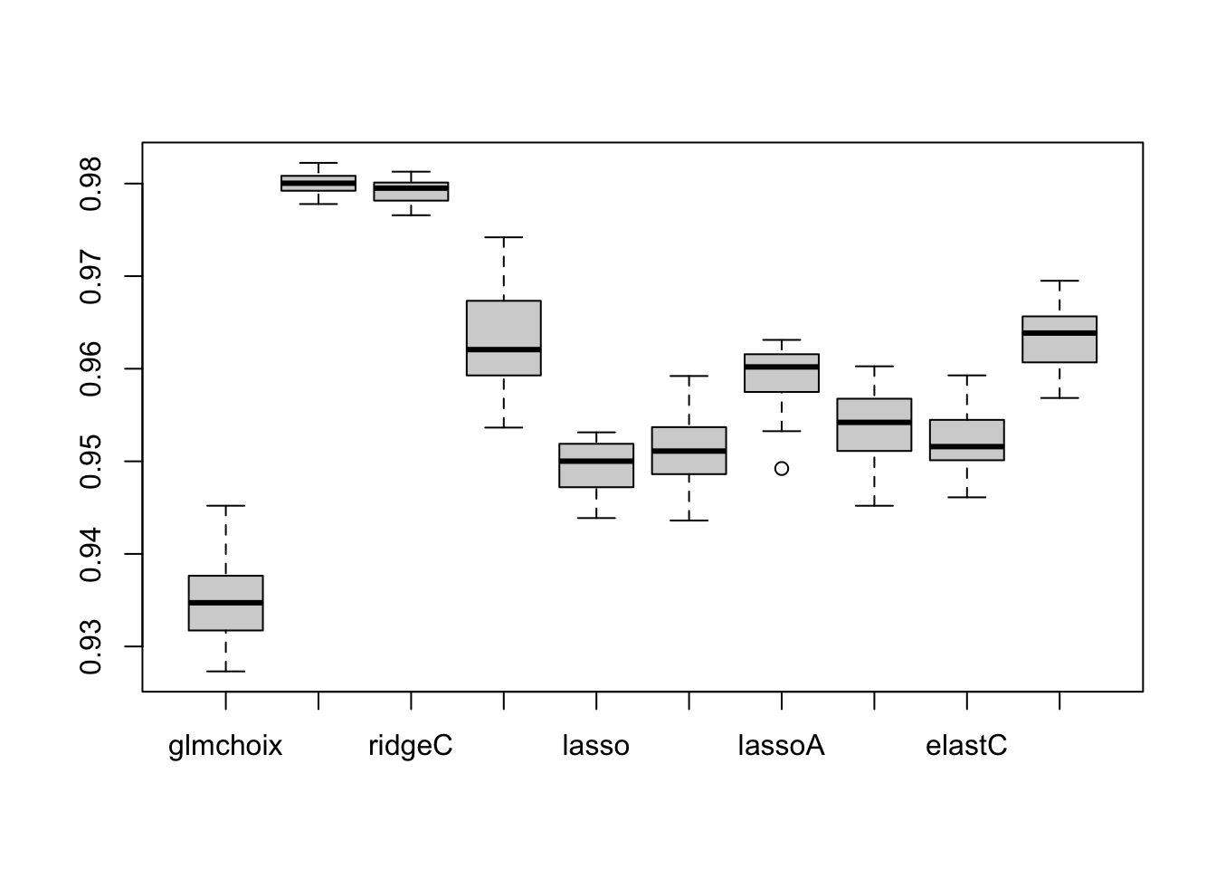

## export 
boxplot(aucm4_20[,-1][,c(1,2,5,8,3,6,9,4,7,10)])